2-Site SFS

The two-site (or two-locus) SFS summarises pairs of linked sites: its entry \((i, j)\) counts pairs of sites, separated by up to d base pairs, at which one site carries \(i\) and the other \(j\) derived alleles. Its departure from the outer product of the one-dimensional spectrum reflects linkage and the shape of the underlying genealogies, which makes it a sensitive probe of departures from the standard (Kingman) coalescent, such as the multiple mergers produced by strong skew in reproductive success (see Fenton et al. [2]).

Setting two_sfs to True makes the Parser pair sites within d base pairs. As with the other parsing modes, parse() returns a TwoSpectra collection keyed by type; without stratifications the single unstratified two-SFS is reached as ["all"], a square TwoSFS. The example uses a synthetic all-sites dataset, monomorphic sites included, simulated under the standard Kingman coalescent.

import sfsutils as su

two_sfs = su.Parser(
    source="resources/msprime/two_sfs_kingman.all.vcf.gz",
    n=10, two_sfs=True, d=1000
).parse()["all"]

INFO:Parser: Using stratification: [all].
INFO:Parser: Loading VCF file
Parser>Counting sites: 600000it [00:00, 4724077.84it/s]
Parser>Processing sites: 100%|██████████| 600000/600000 [03:53<00:00, 2574.77it/s]
INFO:PolyAllelicFiltration: Filtered out 0 sites.
INFO:Parser: Included 600000 out of 600000 sites in total from the input.
INFO:Parser: Counted 299700000 site pairs within 1000 bp.

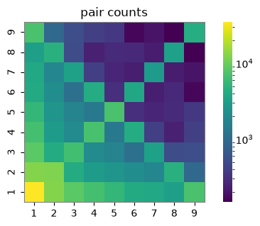
The raw two-site SFS is the symmetric matrix of pair counts, shown here as a heatmap with the monomorphic rows and columns omitted.

two_sfs.plot(title="pair counts");

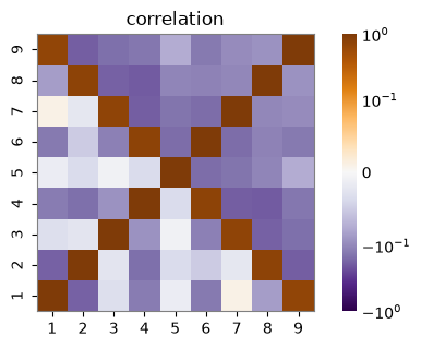
Beyond the raw pair counts, cov() and corr() give the class-resolved branch-length covariance and correlation \(\mathrm{Cov}(L_i, L_j)\) of the two linked sites, the deviation of the joint class distribution from independence. Because they normalise over the whole spectrum so that the marginal is the site-frequency spectrum, they require the monomorphic sites: parse an all-sites input.

two_sfs.corr().plot(title="correlation");

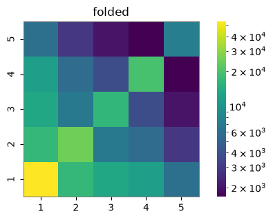
The spectrum can also be folded when the ancestral state is unknown, and the diagonals masked, as for any TwoSFS.

two_sfs.fold().plot(title="folded");

Detecting multiple mergers (MMCs)

Under the Kingman coalescent, mutations at different low frequencies are negatively correlated [3]. Multiple-merger genealogies instead generate positive associations between low-frequency mutations [1], the opposite sign. To see the contrast, we parse a second synthetic all-sites dataset, simulated under a Beta(1.3) multiple-merger coalescent, and compare its correlation with the Kingman one.

beta = su.Parser(
    source="resources/msprime/two_sfs_beta.all.vcf.gz",
    n=10, two_sfs=True, d=1000
).parse()["all"]

INFO:Parser: Using stratification: [all].
INFO:Parser: Loading VCF file
Parser>Counting sites: 600000it [00:00, 4429316.13it/s]
Parser>Processing sites: 100%|██████████| 600000/600000 [04:02<00:00, 2471.72it/s]
INFO:PolyAllelicFiltration: Filtered out 0 sites.
INFO:Parser: Included 600000 out of 600000 sites in total from the input.
INFO:Parser: Counted 299700000 site pairs within 1000 bp.

fig, axes = plt.subplots(1, 2, figsize=(9, 3.6))
two_sfs.corr().plot(ax=axes[0], title="Kingman", show=False)
beta.corr().plot(ax=axes[1], title="Beta(1.3)", show=False)
fig.tight_layout();

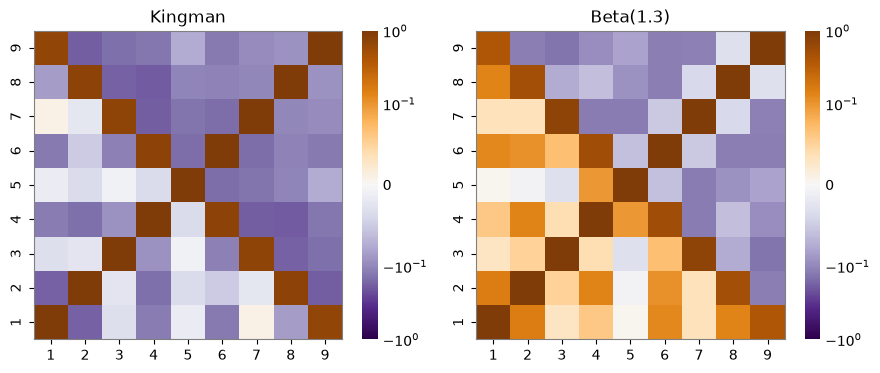
The contrast in the low-frequency block, negative under Kingman and positive under the multiple-merger coalescent, is the signal that two-site spectra exploit to detect departures from Kingman coalescence.

Because cov() and corr() normalise over the full spectrum so that the marginal is the site-frequency spectrum, they require the real monomorphic sites of an all-sites input; a polymorphic-only (SNP) spectrum leaves them undefined and raises. The ratio statistic fpmi() needs no monomorphic sites and remains available for polymorphic-only data. The spectrum can also be folded when the ancestral state is unknown, and the diagonals masked, as for any TwoSFS.